%20(1).png?width=2500&height=1667&name=Portal%20Drop%20Down%20(1)%20(1).png "Take a Tour of Adswerve Connect")
Share


In this blogpost I will show you step by step how to get your GA data into R and do some basic manipulation with that data. The final product will be a heatmap of sessions across 2 dimensions (day of week and hour of day).
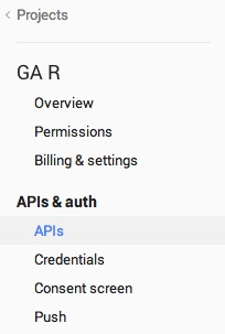
 Create a new project in Google Developers Console[/caption] Open the newly created project inside the console Select APIs from the left navigation and enable Google Analytics API. [caption id="attachment_8877" align="alignnone" width="146"]
 Select APIs from the left menu[/caption] [caption id="attachment_8879" align="alignnone" width="517"]
 Enable Analytics API[/caption]
 Google Analytics View Settings[/caption] [caption id="attachment_8903" align="alignnone" width="422"]
 Make sure to prepend "ga:" to the view ID number when you assign it to the variable. The current example would be "ga:1234567890".[/caption] Now to acquire and validate the token, execute the following code. Note that if the token already exists we will load the existing one.
 Google Analytics Heatmap of sessions by day and hour[/caption]
Step 1: Requirements
To follow this tutorial you will need a Google Analytics account and R software. R is a free software programming language mostly used for statistical purposes and data mining.Step 2: Set up a new Project in Google Developers Console
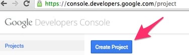
First, open the Google Developers Console
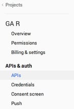
Next, Create a new project [caption id="attachment_8873" align="alignnone" width="389"]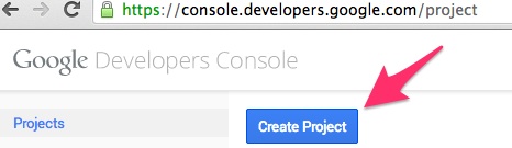 Create a new project in Google Developers Console[/caption] Open the newly created project inside the console Select APIs from the left navigation and enable Google Analytics API. [caption id="attachment_8877" align="alignnone" width="146"]
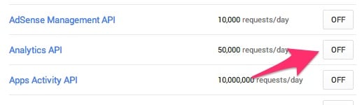
 Select APIs from the left menu[/caption] [caption id="attachment_8879" align="alignnone" width="517"]
 Enable Analytics API[/caption]
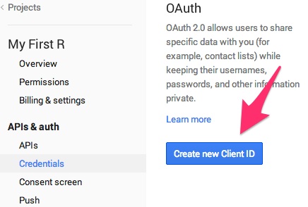
- Under credentials create a new Client Id [caption id="attachment_8881" align="alignnone" width="356"]
 Create new Client ID[/caption] We will be creating a Client ID for an installed application. You will probably need to configure a new consent screen where you will have to pick an email and set a name for the screen. The consent screen is just a page to which the user of your R script will be redirected to authorize access to Google Analytics.
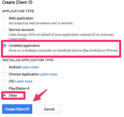
 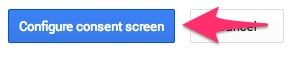 If you followed the steps correctly you should see the following screen. Select "Installed application" and "Other" and then click "Create Client ID". [caption id="attachment_8887" align="alignnone" width="429"]
 Create Client ID[/caption]
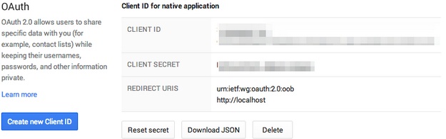
 - On the credentials page of the project you should now see your Client Id and Client Secret. The two strings will be needed to set up your R script to connect to Google Analytics. Leave the page open to copy and paste the values to your R script later.
- [caption id="attachment_8889" align="alignnone" width="625"]
 Leave this page open, you will need Client ID and Client Secret in step 4.[/caption]

Step 3: R Packages
To connect R with Google Analytics API we will be using the RGoogleAnalytics library, which is available on CRAN and can be installed using the following command. Packages that are required for RGoogleAnalytics library to work are lubridate and httr.install.packages("RGoogleAnalytics") Once RGoogleAnalytics library is installed, load the library using “library” or “source” command.
library(RGoogleAnalytics) Install
gplots library which will be used to draw a heatmap the same way.
install.packages("gplots") Once gplots library is installed, load the library using “library” or “source” command.
library(gplots) Last library is
httpuv which simplifies authorization process.
install.packages("httpuv") Once httpuv library is installed, load the library using “library” or “source” command.
library(httpuv)
Step 4: Authorize Access to Google Analytics
After installing all the libraries required for this visualization, first we'll assign the variables to acquire the Google Analytics token. The first two are client.id and client.secret, which should be copy and pasted from the last page in step 2. Client ID and client secret are needed to acquire the oauth token. client.id <- '123456789.apps.googleusercontent.com' client.secret <- 'abcdefghijklmno' view.id <- "ga:1234567890" Third variable (
view.id) is
id of your Google Analytics
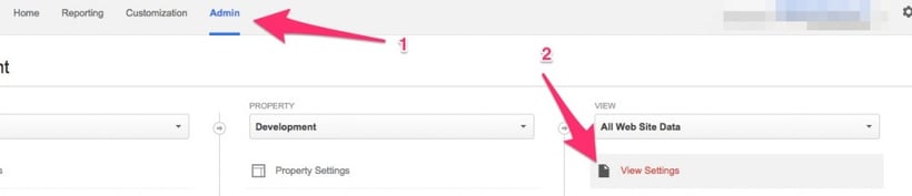
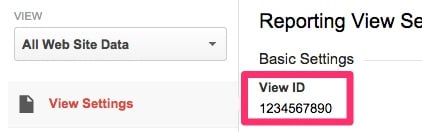
view that you want to visualize. To find your view id, open
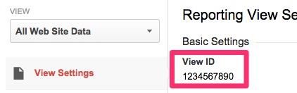
Google Analytics, click "Admin" in the top menu and after you select the desired Account, Property and View, click "View Settings" under the view name. You should now be able to see the view id number. When you assign it to the variable make sure to add "ga:" in front of the number so that it has the following format "ga:1234567890". [caption id="attachment_8901" align="alignnone" width="925"]
 Google Analytics View Settings[/caption] [caption id="attachment_8903" align="alignnone" width="422"]
 Make sure to prepend "ga:" to the view ID number when you assign it to the variable. The current example would be "ga:1234567890".[/caption] Now to acquire and validate the token, execute the following code. Note that if the token already exists we will load the existing one.
if (!file.exists("./token")) {
   token <- Auth(client.id,client.secret)
   token <- save(token,file="./token")
} else {
    load("./token")
}

ValidateToken(token)
Step 5: Google Analytics API Query
Now we can finally connect to Google Analytics and get some data for our view. Let's first set a date range that we'll use in our query. To make this visualization correct, every day of the week should be present the same number of times (use ranges of length 7, 14, 21). Not that first and last day are included in the query.start.date <- "2014-01-26" end.date <- "2014-02-01"Next we set all the query parameters using library's Init function. To understand this better consider playing around with GA Query Explorer. We'll simply query the Google Analytics API with start and end date, dimensions and metrics and view id (set in step 4). Since our heatmap will show the number of sessions according to the day of the week and hour of the day. We query for dimensions ga:hour and ga:dayOfWeek and metric ga:sessions.
query.list <- Init(start.date = start.date,
                   end.date = end.date,
                   dimensions = "ga:hour,ga:dayOfWeek",
                   metrics = "ga:sessions",
                   table.id = view.id)

ga.query <- QueryBuilder(query.list)

ga.data <- GetReportData(ga.query, token)
To get data in R we create a QueryBuilder object out of the query list that we've constructed using the function init and then call GetReportData with the token acquired in the previous step. Our data is then stored in ga.data as a data frame type.
Step 6: Prepare and Clean the data
Now that we have the data, let's clean it and prepare it for the heatmap. To construct a 7 by 24 matrix out of 168 rows of data frame (7days in a week time 24h in a day), we'll convert the sessions column of ga.data data frame into a matrix and then transpose it. Luckily the response from Google Analytics API is already ordered so when we create a matrix with 7 rows, each row will correspond to a day of the week and each of the 24 columns to a certain hour of the day. Transposing the matrix is not necessary, but I've found out that the heatmap looks just a bit nicer this way. To make the visualization more understandable we'll also replace the default matrix row and column names with "human readable" days of the week (Mon, Tue...) and hours of the day (0 to 23).heatmapData <- t(matrix(as.numeric(ga.data$sessions), nrow = 7))
colnames(heatmapData) <- c("Sun", "Mon", "Tue", "Wed", "Thu", "Fri", "Sat")
rownames(heatmapData) <- 0:23
Step 7: Draw the Heatmap
In the last step we'll draw the heatmap. To do this we'll be using heatmap.2 function from the gplots library.heatmap.2(heatmapData, dendrogram="none", Rowv = NA, Colv=NA, col=cm.colors(20), margins=c(5,10), scale="none", trace="none", denscol="red", key.title="", key.xlab = "Sessions")You can manipulate the visualization using the heatmap.2 parameters. To see what each parameter can do, type ?heatmap.2 in your R console. The ones that I've used omit drawing a dendrogram (which is by default a part of the heatmap). Avoid sorting by row and column ( Colv, RowvB). Use different color set, add a margin, scale according to the min and max value of the entire matrix (and not by individual row or column). Avoid drawing a trace in heatmap. Change the color of the histogram in the legend to make it better visible ( denscol), and change some text ( key.title and key.xlab).
The Final Result
The final result is a useful heatmap that helps identify what time and which days our website is most popular. The interpretation of the following heatmap indicates that our website has very few visitors during the weekends (blue), and is most popular on weekdays between 11 and 16 (4PM). The little legend on the top left also includes a histogram of sessions per hour. [caption id="attachment_8895" align="alignnone" width="668"]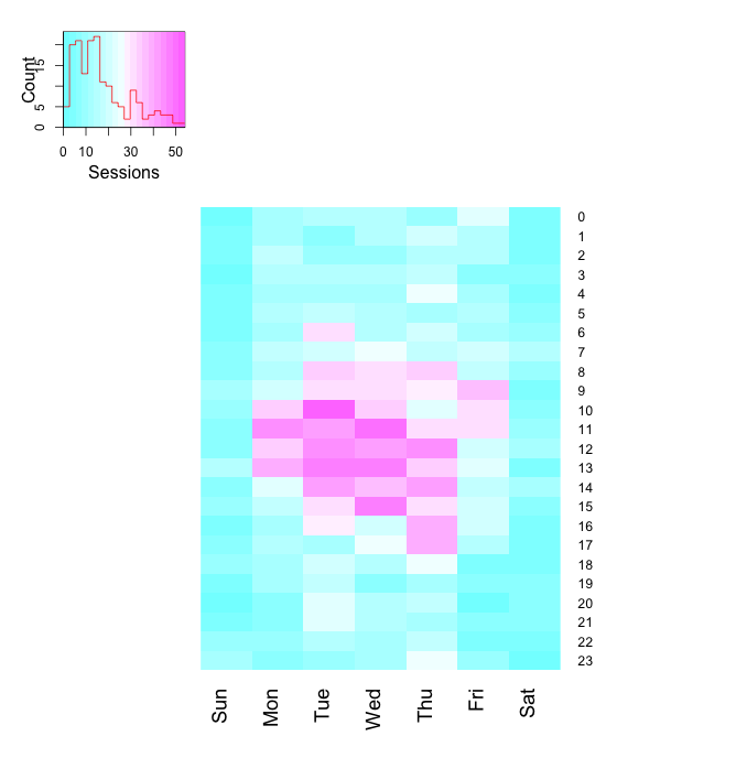 Google Analytics Heatmap of sessions by day and hour[/caption]